Hypothesis testing have been extensively used on different discipline of science. And in this post, I will attempt on discussing the basic theory behind this, the Likelihood Ratio Test (LRT) defined below from Casella and Berger (2001), see reference 1.
Example 1. Let $X_1,X_2,\cdots,X_n\overset{r.s.}{\sim}f(x|\theta)=\frac{1}{\theta}\exp\left[-\frac{x}{\theta}\right],x>0,\theta>0$. From this sample, consider testing $H_0:\theta = \theta_0$ vs $H_1:\theta<\theta_0$.
Solution:
The parameter space $\Theta$ is the set $(0,\Theta_0]$, where $\Theta_0=\{\theta_0\}$. Hence, using the likelihood ratio test, we have $$ \lambda(\mathbf{x})=\frac{\displaystyle\sup_{\theta=\theta_0}L(\theta|\mathbf{x})}{\displaystyle\sup_{\theta\leq\theta_0}L(\theta|\mathbf{x})}, $$ where, $$ \begin{aligned} \sup_{\theta=\theta_0}L(\theta|\mathbf{x})&=\sup_{\theta=\theta_0}\prod_{i=1}^{n}\frac{1}{\theta}\exp\left[-\frac{x_i}{\theta}\right]\\ &=\sup_{\theta=\theta_0}\left(\frac{1}{\theta}\right)^n\exp\left[-\displaystyle\frac{\sum_{i=1}^{n}x_i}{\theta}\right]\\ &=\left(\frac{1}{\theta_0}\right)^n\exp\left[-\displaystyle\frac{\sum_{i=1}^{n}x_i}{\theta_0}\right], \end{aligned} $$ and $$ \begin{aligned} \sup_{\theta\leq\theta_0}L(\theta|\mathbf{x})&=\sup_{\theta\leq\theta_0}\prod_{i=1}^{n}\frac{1}{\theta}\exp\left[-\frac{x_i}{\theta}\right]\\ &=\sup_{\theta\leq\theta_0}\left(\frac{1}{\theta}\right)^n\exp\left[-\displaystyle\frac{\sum_{i=1}^{n}x_i}{\theta}\right]=\sup_{\theta\leq\theta_0}f(\mathbf{x}|\theta). \end{aligned} $$ Now the supremum of $f(\mathbf{x}|\theta)$ over all values of $\theta\leq\theta_0$ is the MLE (maximum likelihood estimator) of $f(x|\theta)$, which is $\bar{x}$, provided that $\bar{x}\leq \theta_0$.
So that, $$ \begin{aligned} \lambda(\mathbf{x})&=\frac{\left(\frac{1}{\theta_0}\right)^n\exp\left[-\displaystyle\frac{\sum_{i=1}^{n}x_i}{\theta_0}\right]} {\left(\frac{1}{\bar{x}}\right)^n\exp\left[-\displaystyle\frac{\sum_{i=1}^{n}x_i}{\bar{x}}\right]},\quad\text{provided that}\;\bar{x}\leq \theta_0\\ &=\left(\frac{\bar{x}}{\theta_0}\right)^n\exp\left[-\displaystyle\frac{\sum_{i=1}^{n}x_i}{\theta_0}\right]\exp[n]. \end{aligned} $$ And we say that, if $\lambda(\mathbf{x})\leq c$, $H_0$ is rejected. That is, $$ \begin{aligned} \left(\frac{\bar{x}}{\theta_0}\right)^n\exp\left[-\displaystyle\frac{\sum_{i=1}^{n}x_i}{\theta_0}\right]\exp[n]&\leq c\\ \left(\frac{\bar{x}}{\theta_0}\right)^n\exp\left[-\displaystyle\frac{\sum_{i=1}^{n}x_i}{\theta_0}\right]&\leq c',\quad\text{where}\;c'=\frac{c}{\exp[n]}\\ n\log\left(\frac{\bar{x}}{\theta_0}\right)-\frac{n}{\theta_0}\bar{x}&\leq \log c'\\ \log\left(\frac{\bar{x}}{\theta_0}\right)-\frac{\bar{x}}{\theta_0}&\leq \frac{1}{n}\log c'\\ \log\left(\frac{\bar{x}}{\theta_0}\right)-\frac{\bar{x}}{\theta_0}&\leq \frac{1}{n}\log c-1. \end{aligned} $$ Now let $h(x)=\log x - x$, then $h'(x)=\frac{1}{x}-1$. So the critical point of $h'(x)$ is $x=1$. And to test if this is maximum or minimum, we apply second derivative test. That is, $$ h''(x)=-\frac{1}{x^2}<0,\forall x. $$ Thus, $x=1$ is a maximum. Hence, $ \log\left(\frac{\bar{x}}{\theta_0}\right)-\frac{\bar{x}}{\theta_0} $ is maximized if $\frac{\bar{x}}{\theta_0}=1\Rightarrow\bar{x}=\theta_0$. To see this consider the following plot,
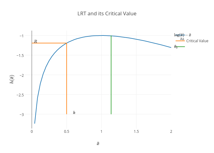 Above figure is the plot of $h(\bar{x})$ function with $\theta_0=1$. Given the assumption that $\bar{x}\leq \theta_0$ then assuming $R=\frac{1}{n}\log c-1$ designates the orange line above, then we reject $H_0$ if $h(\bar{x})\leq R$, if and only if $\bar{x}\leq k$. In practice, $k$ is specified to satisfy,
$$
\mathrm{P}(\bar{x}\leq k|\theta=\theta_0)\leq \alpha,
$$
where $\alpha$ is called the level of the test.
Above figure is the plot of $h(\bar{x})$ function with $\theta_0=1$. Given the assumption that $\bar{x}\leq \theta_0$ then assuming $R=\frac{1}{n}\log c-1$ designates the orange line above, then we reject $H_0$ if $h(\bar{x})\leq R$, if and only if $\bar{x}\leq k$. In practice, $k$ is specified to satisfy,
$$
\mathrm{P}(\bar{x}\leq k|\theta=\theta_0)\leq \alpha,
$$
where $\alpha$ is called the level of the test.
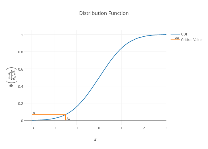
It follows that $X_i|\theta = \theta_0\overset{r.s.}{\sim}\exp[\theta_0]$, then $\mathrm{E}X_i=\theta_0$ and $\mathrm{Var}X_i=\theta_0^2$. If $\bar{x}=\frac{1}{n}\sum_{i=1}^{n}X_i$ and if $G_n$ is the distribution of $\frac{(\bar{x}_n-\theta_0)}{\sqrt{\frac{\theta_0^2}{n}}}$. By CLT (central limit theorem) $\lim_{n\to\infty}G_n$ converges to standard normal distribution. That is, $\bar{x}|\theta = \theta_0\overset{r.s.}{\sim}AN\left(\theta_0,\frac{\theta_0^2}{n}\right)$. $AN$ - assymptotically normal.
Thus, $$ \mathrm{P}(\bar{x}\leq k|\theta=\theta_0)=\Phi\left(\frac{k-\theta_0}{\theta_0/\sqrt{n}}\right),\quad\text{for large }n. $$ So that, $$ \mathrm{P}(\bar{x}\leq k|\theta=\theta_0)=\Phi\left(\frac{k-\theta_0}{\theta_0/\sqrt{n}}\right)\leq \alpha. $$ Plotting this gives us,
 with corresponding PDF given by,
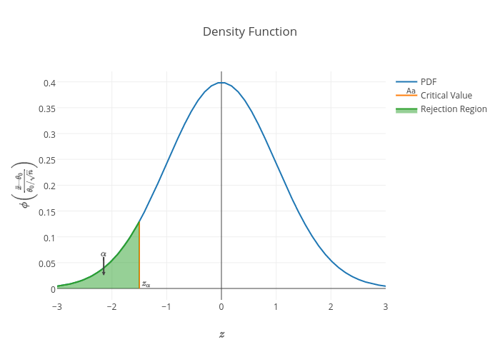 Implying,
$$
\frac{k-\theta_0}{\theta_0/\sqrt{n}}=z_{\alpha}\Rightarrow k=\theta_0+z_{\alpha}\frac{\theta_0}{\sqrt{n}}.
$$
Therefore, a level-$\alpha$ test of $H_0:\theta=\theta_0$ vs $H_1:\theta<\theta_0$ is the test that rejects $H_0$ when $\bar{x}\leq\theta_0+z_{\alpha}\frac{\theta_0}{\sqrt{n}}$.
Implying,
$$
\frac{k-\theta_0}{\theta_0/\sqrt{n}}=z_{\alpha}\Rightarrow k=\theta_0+z_{\alpha}\frac{\theta_0}{\sqrt{n}}.
$$
Therefore, a level-$\alpha$ test of $H_0:\theta=\theta_0$ vs $H_1:\theta<\theta_0$ is the test that rejects $H_0$ when $\bar{x}\leq\theta_0+z_{\alpha}\frac{\theta_0}{\sqrt{n}}$.
Definition. The likelihood ratio test statistic for testing $H_0:\theta\in\Theta_0$ versus $H_1:\theta\in\Theta_0^c$ is \begin{equation} \label{eq:lrt} \lambda(\mathbf{x})=\frac{\displaystyle\sup_{\theta\in\Theta_0}L(\theta|\mathbf{x})}{\displaystyle\sup_{\theta\in\Theta}L(\theta|\mathbf{x})}. \end{equation} A likelihood ratio test (LRT) is any test that has a rejection region of the form $\{\mathbf{x}:\lambda(\mathbf{x})\leq c\}$, where $c$ is any number satisfying $0\leq c \leq 1$.The numerator of equation (\ref{eq:lrt}) gives us the supremum probability of the parameter, $\theta$, over the restricted domain (null hypothesis, $\Theta_0$) of the parameter space $\Theta$, that maximizes the joint probability of the sample, $\mathbf{x}$. While the denominator of the LRT gives us the supremum probability of the parameter, $\theta$, over the unrestricted domain, $\Theta$, that maximizes the joint probability of the sample, $\mathbf{x}$. Therefore, if the value of $\lambda(\mathbf{x})$ is small such that $\lambda(\mathbf{x})\leq c$, for some $c\in [0, 1]$, then the true value of the parameter that is plausible in explaining the sample is likely to be in the alternative hypothesis, $\Theta_0^c$.
Example 1. Let $X_1,X_2,\cdots,X_n\overset{r.s.}{\sim}f(x|\theta)=\frac{1}{\theta}\exp\left[-\frac{x}{\theta}\right],x>0,\theta>0$. From this sample, consider testing $H_0:\theta = \theta_0$ vs $H_1:\theta<\theta_0$.
Solution:
The parameter space $\Theta$ is the set $(0,\Theta_0]$, where $\Theta_0=\{\theta_0\}$. Hence, using the likelihood ratio test, we have $$ \lambda(\mathbf{x})=\frac{\displaystyle\sup_{\theta=\theta_0}L(\theta|\mathbf{x})}{\displaystyle\sup_{\theta\leq\theta_0}L(\theta|\mathbf{x})}, $$ where, $$ \begin{aligned} \sup_{\theta=\theta_0}L(\theta|\mathbf{x})&=\sup_{\theta=\theta_0}\prod_{i=1}^{n}\frac{1}{\theta}\exp\left[-\frac{x_i}{\theta}\right]\\ &=\sup_{\theta=\theta_0}\left(\frac{1}{\theta}\right)^n\exp\left[-\displaystyle\frac{\sum_{i=1}^{n}x_i}{\theta}\right]\\ &=\left(\frac{1}{\theta_0}\right)^n\exp\left[-\displaystyle\frac{\sum_{i=1}^{n}x_i}{\theta_0}\right], \end{aligned} $$ and $$ \begin{aligned} \sup_{\theta\leq\theta_0}L(\theta|\mathbf{x})&=\sup_{\theta\leq\theta_0}\prod_{i=1}^{n}\frac{1}{\theta}\exp\left[-\frac{x_i}{\theta}\right]\\ &=\sup_{\theta\leq\theta_0}\left(\frac{1}{\theta}\right)^n\exp\left[-\displaystyle\frac{\sum_{i=1}^{n}x_i}{\theta}\right]=\sup_{\theta\leq\theta_0}f(\mathbf{x}|\theta). \end{aligned} $$ Now the supremum of $f(\mathbf{x}|\theta)$ over all values of $\theta\leq\theta_0$ is the MLE (maximum likelihood estimator) of $f(x|\theta)$, which is $\bar{x}$, provided that $\bar{x}\leq \theta_0$.
So that, $$ \begin{aligned} \lambda(\mathbf{x})&=\frac{\left(\frac{1}{\theta_0}\right)^n\exp\left[-\displaystyle\frac{\sum_{i=1}^{n}x_i}{\theta_0}\right]} {\left(\frac{1}{\bar{x}}\right)^n\exp\left[-\displaystyle\frac{\sum_{i=1}^{n}x_i}{\bar{x}}\right]},\quad\text{provided that}\;\bar{x}\leq \theta_0\\ &=\left(\frac{\bar{x}}{\theta_0}\right)^n\exp\left[-\displaystyle\frac{\sum_{i=1}^{n}x_i}{\theta_0}\right]\exp[n]. \end{aligned} $$ And we say that, if $\lambda(\mathbf{x})\leq c$, $H_0$ is rejected. That is, $$ \begin{aligned} \left(\frac{\bar{x}}{\theta_0}\right)^n\exp\left[-\displaystyle\frac{\sum_{i=1}^{n}x_i}{\theta_0}\right]\exp[n]&\leq c\\ \left(\frac{\bar{x}}{\theta_0}\right)^n\exp\left[-\displaystyle\frac{\sum_{i=1}^{n}x_i}{\theta_0}\right]&\leq c',\quad\text{where}\;c'=\frac{c}{\exp[n]}\\ n\log\left(\frac{\bar{x}}{\theta_0}\right)-\frac{n}{\theta_0}\bar{x}&\leq \log c'\\ \log\left(\frac{\bar{x}}{\theta_0}\right)-\frac{\bar{x}}{\theta_0}&\leq \frac{1}{n}\log c'\\ \log\left(\frac{\bar{x}}{\theta_0}\right)-\frac{\bar{x}}{\theta_0}&\leq \frac{1}{n}\log c-1. \end{aligned} $$ Now let $h(x)=\log x - x$, then $h'(x)=\frac{1}{x}-1$. So the critical point of $h'(x)$ is $x=1$. And to test if this is maximum or minimum, we apply second derivative test. That is, $$ h''(x)=-\frac{1}{x^2}<0,\forall x. $$ Thus, $x=1$ is a maximum. Hence, $ \log\left(\frac{\bar{x}}{\theta_0}\right)-\frac{\bar{x}}{\theta_0} $ is maximized if $\frac{\bar{x}}{\theta_0}=1\Rightarrow\bar{x}=\theta_0$. To see this consider the following plot,
It follows that $X_i|\theta = \theta_0\overset{r.s.}{\sim}\exp[\theta_0]$, then $\mathrm{E}X_i=\theta_0$ and $\mathrm{Var}X_i=\theta_0^2$. If $\bar{x}=\frac{1}{n}\sum_{i=1}^{n}X_i$ and if $G_n$ is the distribution of $\frac{(\bar{x}_n-\theta_0)}{\sqrt{\frac{\theta_0^2}{n}}}$. By CLT (central limit theorem) $\lim_{n\to\infty}G_n$ converges to standard normal distribution. That is, $\bar{x}|\theta = \theta_0\overset{r.s.}{\sim}AN\left(\theta_0,\frac{\theta_0^2}{n}\right)$. $AN$ - assymptotically normal.
Thus, $$ \mathrm{P}(\bar{x}\leq k|\theta=\theta_0)=\Phi\left(\frac{k-\theta_0}{\theta_0/\sqrt{n}}\right),\quad\text{for large }n. $$ So that, $$ \mathrm{P}(\bar{x}\leq k|\theta=\theta_0)=\Phi\left(\frac{k-\theta_0}{\theta_0/\sqrt{n}}\right)\leq \alpha. $$ Plotting this gives us,
Comments
Post a Comment