In my previous article, we talked about implementations of linear regression models in R, Python and SAS. On the theoretical sides, however, I briefly mentioned the estimation procedure for the parameter $\boldsymbol{\beta}$. So to help us understand how software does the estimation procedure, we'll look at the mathematics behind it. We will also perform the estimation manually in R and in Python, that means we're not going to use any special packages, this will help us appreciate the theory.
 Performing differentiation under $(p+1)$-dimensional parameter $\boldsymbol{\beta}$ is manageable in the context of linear algebra, so Equation (\ref{eq:2}) is equivalent to
\begin{align*}
\lVert\mathbf{y}-\mathbf{X}\boldsymbol{\beta}\rVert^2&=\langle\mathbf{y}-\mathbf{X}\boldsymbol{\beta},\mathbf{y}-\mathbf{X}\boldsymbol{\beta}\rangle=\mathbf{y}^{\text{T}}\mathbf{y}-\mathbf{y}^{\text{T}}\mathbf{X}\boldsymbol{\beta}-(\mathbf{X}\boldsymbol{\beta})^{\text{T}}\mathbf{y}+(\mathbf{X}\boldsymbol{\beta})^{\text{T}}\mathbf{X}\boldsymbol{\beta}\\
&=\mathbf{y}^{\text{T}}\mathbf{y}-\mathbf{y}^{\text{T}}\mathbf{X}\boldsymbol{\beta}-\boldsymbol{\beta}^{\text{T}}\mathbf{X}^{\text{T}}\mathbf{y}+\boldsymbol{\beta}^{\text{T}}\mathbf{X}^{\text{T}}\mathbf{X}\boldsymbol{\beta}
\end{align*}
And the derivative with respect to the parameter is
\begin{align*}
\frac{\operatorname{\partial}}{\operatorname{\partial}\boldsymbol{\beta}}\lVert\mathbf{y}-\mathbf{X}\boldsymbol{\beta}\rVert^2&=-2\mathbf{X}^{\text{T}}\mathbf{y}+2\mathbf{X}^{\text{T}}\mathbf{X}\boldsymbol{\beta}
\end{align*}
Taking the critical point by setting the above equation to zero vector, we have
\begin{align}
\frac{\operatorname{\partial}}{\operatorname{\partial}\boldsymbol{\beta}}\lVert\mathbf{y}-\mathbf{X}\hat{\boldsymbol{\beta}}\rVert^2&\overset{\text{set}}{=}\mathbf{0}\nonumber\\
-\mathbf{X}^{\text{T}}\mathbf{y}+\mathbf{X}^{\text{T}}\mathbf{X}\hat{\boldsymbol{\beta}}&=\mathbf{0}\nonumber\\
\mathbf{X}^{\text{T}}\mathbf{X}\hat{\boldsymbol{\beta}}&=\mathbf{X}^{\text{T}}\mathbf{y}\label{eq:norm}
\end{align}
Equation (\ref{eq:norm}) is called the normal equation. If $\mathbf{X}$ is full rank, then we can compute the inverse of $\mathbf{X}^{\text{T}}\mathbf{X}$,
\begin{align}
\mathbf{X}^{\text{T}}\mathbf{X}\hat{\boldsymbol{\beta}}&=\mathbf{X}^{\text{T}}\mathbf{y}\nonumber\\
(\mathbf{X}^{\text{T}}\mathbf{X})^{-1}\mathbf{X}^{\text{T}}\mathbf{X}\hat{\boldsymbol{\beta}}&=(\mathbf{X}^{\text{T}}\mathbf{X})^{-1}\mathbf{X}^{\text{T}}\mathbf{y}\nonumber\\
\hat{\boldsymbol{\beta}}&=(\mathbf{X}^{\text{T}}\mathbf{X})^{-1}\mathbf{X}^{\text{T}}\mathbf{y}.\label{eq:betahat}
\end{align}
That's it, since both $\mathbf{X}$ and $\mathbf{y}$ are known.
Performing differentiation under $(p+1)$-dimensional parameter $\boldsymbol{\beta}$ is manageable in the context of linear algebra, so Equation (\ref{eq:2}) is equivalent to
\begin{align*}
\lVert\mathbf{y}-\mathbf{X}\boldsymbol{\beta}\rVert^2&=\langle\mathbf{y}-\mathbf{X}\boldsymbol{\beta},\mathbf{y}-\mathbf{X}\boldsymbol{\beta}\rangle=\mathbf{y}^{\text{T}}\mathbf{y}-\mathbf{y}^{\text{T}}\mathbf{X}\boldsymbol{\beta}-(\mathbf{X}\boldsymbol{\beta})^{\text{T}}\mathbf{y}+(\mathbf{X}\boldsymbol{\beta})^{\text{T}}\mathbf{X}\boldsymbol{\beta}\\
&=\mathbf{y}^{\text{T}}\mathbf{y}-\mathbf{y}^{\text{T}}\mathbf{X}\boldsymbol{\beta}-\boldsymbol{\beta}^{\text{T}}\mathbf{X}^{\text{T}}\mathbf{y}+\boldsymbol{\beta}^{\text{T}}\mathbf{X}^{\text{T}}\mathbf{X}\boldsymbol{\beta}
\end{align*}
And the derivative with respect to the parameter is
\begin{align*}
\frac{\operatorname{\partial}}{\operatorname{\partial}\boldsymbol{\beta}}\lVert\mathbf{y}-\mathbf{X}\boldsymbol{\beta}\rVert^2&=-2\mathbf{X}^{\text{T}}\mathbf{y}+2\mathbf{X}^{\text{T}}\mathbf{X}\boldsymbol{\beta}
\end{align*}
Taking the critical point by setting the above equation to zero vector, we have
\begin{align}
\frac{\operatorname{\partial}}{\operatorname{\partial}\boldsymbol{\beta}}\lVert\mathbf{y}-\mathbf{X}\hat{\boldsymbol{\beta}}\rVert^2&\overset{\text{set}}{=}\mathbf{0}\nonumber\\
-\mathbf{X}^{\text{T}}\mathbf{y}+\mathbf{X}^{\text{T}}\mathbf{X}\hat{\boldsymbol{\beta}}&=\mathbf{0}\nonumber\\
\mathbf{X}^{\text{T}}\mathbf{X}\hat{\boldsymbol{\beta}}&=\mathbf{X}^{\text{T}}\mathbf{y}\label{eq:norm}
\end{align}
Equation (\ref{eq:norm}) is called the normal equation. If $\mathbf{X}$ is full rank, then we can compute the inverse of $\mathbf{X}^{\text{T}}\mathbf{X}$,
\begin{align}
\mathbf{X}^{\text{T}}\mathbf{X}\hat{\boldsymbol{\beta}}&=\mathbf{X}^{\text{T}}\mathbf{y}\nonumber\\
(\mathbf{X}^{\text{T}}\mathbf{X})^{-1}\mathbf{X}^{\text{T}}\mathbf{X}\hat{\boldsymbol{\beta}}&=(\mathbf{X}^{\text{T}}\mathbf{X})^{-1}\mathbf{X}^{\text{T}}\mathbf{y}\nonumber\\
\hat{\boldsymbol{\beta}}&=(\mathbf{X}^{\text{T}}\mathbf{X})^{-1}\mathbf{X}^{\text{T}}\mathbf{y}.\label{eq:betahat}
\end{align}
That's it, since both $\mathbf{X}$ and $\mathbf{y}$ are known.
R Script Python Script Here we have two predictors
 Now let's estimate the parameter $\boldsymbol{\beta}$ which by default we set to $\beta_1=3.5$ and $\beta_2=2.8$. We will use Equation (\ref{eq:betahat}) for estimation. So that we have
R Script Python Script That's a good estimate, and again just a reminder, the estimate in R and in Python are different because we have different random samples, the important thing is that both are iid. To proceed, we'll do prediction using Equations (\ref{eq:pred}). That is,
R Script Python Script The first column above is the data
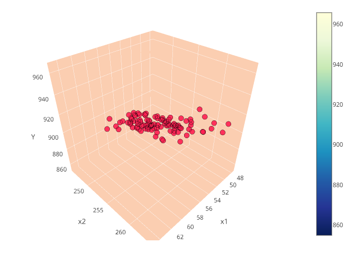 You have to rotate the plot by the way to see the plane, I still can't figure out how to change it in Plotly. Anyway, at this point we can proceed computing for other statistics like the variance of the error, and so on. But I will leave it for you to explore. Our aim here is just to give us an understanding on what is happening inside the internals of our software when we try to estimate the parameters of the linear regression models.
Linear Least Squares
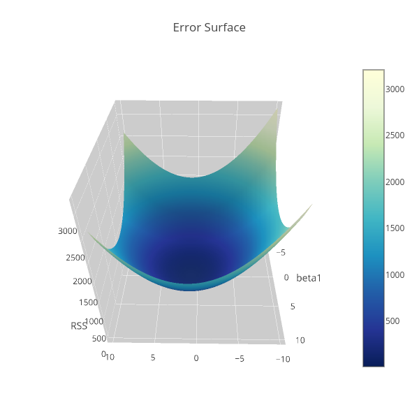
Consider the linear regression model, \[ y_i=f_i(\mathbf{x}|\boldsymbol{\beta})+\varepsilon_i,\quad\mathbf{x}_i=\left[ \begin{array}{cccc} 1&x_{11}&\cdots&x_{1p} \end{array}\right],\quad\boldsymbol{\beta}=\left[\begin{array}{c}\beta_0\\\beta_1\\\vdots\\\beta_p\end{array}\right], \] where $y_i$ is the response or the dependent variable at the $i$th case, $i=1,\cdots, N$. The $f_i(\mathbf{x}|\boldsymbol{\beta})$ is the deterministic part of the model that depends on both the parameters $\boldsymbol{\beta}\in\mathbb{R}^{p+1}$ and the predictor variable $\mathbf{x}_i$, which in matrix form, say $\mathbf{X}$, is represented as follows \[ \mathbf{X}=\left[ \begin{array}{cccccc} 1&x_{11}&\cdots&x_{1p}\\ 1&x_{21}&\cdots&x_{2p}\\ \vdots&\vdots&\ddots&\vdots\\ 1&x_{N1}&\cdots&x_{Np}\\ \end{array} \right]. \] $\varepsilon_i$ is the error term at the $i$th case which we assumed to be Gaussian distributed with mean 0 and variance $\sigma^2$. So that \[ \mathbb{E}y_i=f_i(\mathbf{x}|\boldsymbol{\beta}), \] i.e. $f_i(\mathbf{x}|\boldsymbol{\beta})$ is the expectation function. The uncertainty around the response variable is also modelled by Gaussian distribution. Specifically, if $Y=f(\mathbf{x}|\boldsymbol{\beta})+\varepsilon$ and $y\in Y$ such that $y>0$, then \begin{align*} \mathbb{P}[Y\leq y]&=\mathbb{P}[f(x|\beta)+\varepsilon\leq y]\\ &=\mathbb{P}[\varepsilon\leq y-f(\mathbf{x}|\boldsymbol{\beta})]=\mathbb{P}\left[\frac{\varepsilon}{\sigma}\leq \frac{y-f(\mathbf{x}|\boldsymbol{\beta})}{\sigma}\right]\\ &=\Phi\left[\frac{y-f(\mathbf{x}|\boldsymbol{\beta})}{\sigma}\right], \end{align*} where $\Phi$ denotes the Gaussian distribution with density denoted by $\phi$ below. Hence $Y\sim\mathcal{N}(f(\mathbf{x}|\boldsymbol{\beta}),\sigma^2)$. That is, \begin{align*} \frac{\operatorname{d}}{\operatorname{d}y}\Phi\left[\frac{y-f(\mathbf{x}|\boldsymbol{\beta})}{\sigma}\right]&=\phi\left[\frac{y-f(\mathbf{x}|\boldsymbol{\beta})}{\sigma}\right]\frac{1}{\sigma}=\mathbb{P}[y|f(\mathbf{x}|\boldsymbol{\beta}),\sigma^2]\\ &=\frac{1}{\sqrt{2\pi}\sigma}\exp\left\{-\frac{1}{2}\left[\frac{y-f(\mathbf{x}|\boldsymbol{\beta})}{\sigma}\right]^2\right\}. \end{align*} If the data are independent and identically distributed, then the log-likelihood function of $y$ is, \begin{align*} \mathcal{L}[\boldsymbol{\beta}|\mathbf{y},\mathbf{X},\sigma]&=\mathbb{P}[\mathbf{y}|\mathbf{X},\boldsymbol{\beta},\sigma]=\prod_{i=1}^N\frac{1}{\sqrt{2\pi}\sigma}\exp\left\{-\frac{1}{2}\left[\frac{y_i-f_i(\mathbf{x}|\boldsymbol{\beta})}{\sigma}\right]^2\right\}\\ &=\frac{1}{(2\pi)^{\frac{n}{2}}\sigma^n}\exp\left\{-\frac{1}{2}\sum_{i=1}^N\left[\frac{y_i-f_i(\mathbf{x}|\boldsymbol{\beta})}{\sigma}\right]^2\right\}\\ \log\mathcal{L}[\boldsymbol{\beta}|\mathbf{y},\mathbf{X},\sigma]&=-\frac{n}{2}\log2\pi-n\log\sigma-\frac{1}{2\sigma^2}\sum_{i=1}^N\left[y_i-f_i(\mathbf{x}|\boldsymbol{\beta})\right]^2. \end{align*} And because the likelihood function tells us about the plausibility of the parameter $\boldsymbol{\beta}$ in explaining the sample data. We therefore want to find the best estimate of $\boldsymbol{\beta}$ that likely generated the sample. Thus our goal is to maximize the likelihood function which is equivalent to maximizing the log-likelihood with respect to $\boldsymbol{\beta}$. And that's simply done by taking the partial derivative with respect to the parameter $\boldsymbol{\beta}$. Therefore, the first two terms in the right hand side of the equation above can be disregarded since it does not depend on $\boldsymbol{\beta}$. Also, the location of the maximum log-likelihood with respect to $\boldsymbol{\beta}$ is not affected by arbitrary positive scalar multiplication, so the factor $\frac{1}{2\sigma^2}$ can be omitted. And we are left with the following equation, \begin{equation}\label{eq:1} -\sum_{i=1}^N\left[y_i-f_i(\mathbf{x}|\boldsymbol{\beta})\right]^2. \end{equation} One last thing is that, instead of maximizing the log-likelihood function we can do minimization on the negative log-likelihood. Hence we are interested on minimizing the negative of Equation (\ref{eq:1}) which is \begin{equation}\label{eq:2} \sum_{i=1}^N\left[y_i-f_i(\mathbf{x}|\boldsymbol{\beta})\right]^2, \end{equation} popularly known as the residual sum of squares (RSS). So RSS is a consequence of maximum log-likelihood under the Gaussian assumption of the uncertainty around the response variable $y$. For models with two parameters, say $\beta_0$ and $\beta_1$ the RSS can be visualized like the one in my previous article, that is
Prediction
If $\mathbf{X}$ is full rank and spans the subspace $V\subseteq\mathbb{R}^N$, where $\mathbb{E}\mathbf{y}=\mathbf{X}\boldsymbol{\beta}\in V$. Then the predicted values of $\mathbf{y}$ is given by, \begin{equation}\label{eq:pred} \hat{\mathbf{y}}=\mathbb{E}\mathbf{y}=\mathbf{P}_{V}\mathbf{y}=\mathbf{X}(\mathbf{X}^{\text{T}}\mathbf{X})^{-1}\mathbf{X}^{\text{T}}\mathbf{y}, \end{equation} where $\mathbf{P}$ is the projection matrix onto the space $V$. For proof of the projection matrix in Equation (\ref{eq:pred}) please refer to reference (1) below. Notice that this is equivalent to \begin{equation}\label{eq:yhbh} \hat{\mathbf{y}}=\mathbb{E}\mathbf{y}=\mathbf{X}\hat{\boldsymbol{\beta}}. \end{equation}Computation
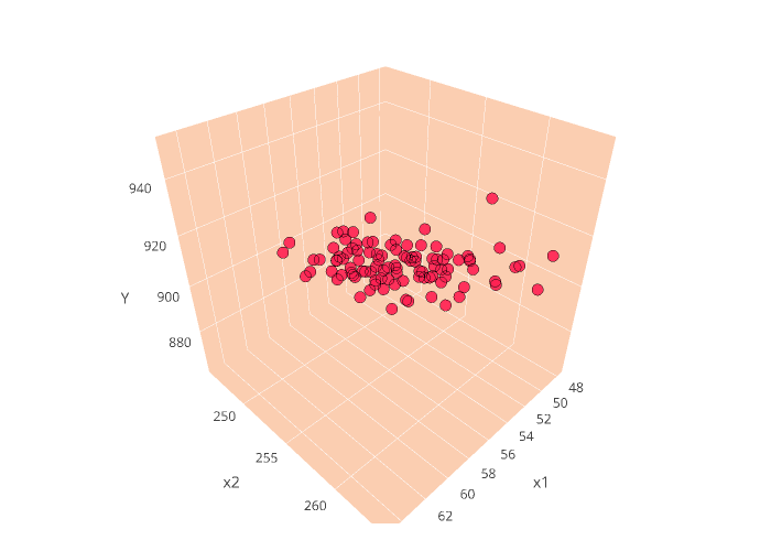
Let's fire up R and Python and see how we can apply those equations we derived. For purpose of illustration, we're going to simulate data from Gaussian distributed population. To do so, consider the following codesR Script Python Script Here we have two predictors
x1 and x2, and our response variable y is generated by the parameters $\beta_1=3.5$ and $\beta_2=2.8$, and it has Gaussian noise with variance 7. While we set the same random seeds for both R and Python, we should not expect the random values generated in both languages to be identical, instead both values are independent and identically distributed (iid). For visualization, I will use Python Plotly, you can also translate it to R Plotly.
R Script Python Script That's a good estimate, and again just a reminder, the estimate in R and in Python are different because we have different random samples, the important thing is that both are iid. To proceed, we'll do prediction using Equations (\ref{eq:pred}). That is,
R Script Python Script The first column above is the data
y and the second column is the prediction due to Equation (\ref{eq:pred}). Thus if we are to expand the prediction into an expectation plane, then we have
Reference
- Arnold, Steven F. (1981). The Theory of Linear Models and Multivariate Analysis. Wiley.
- OLS in Matrix Form
Comments
Post a Comment