Analysis with Programming has recently been syndicated to Planet Python. And as a first post being a contributing blog on the said site, I would like to share how to get started with data analysis on Python. Specifically, I would like to do the following:
To read CSV file locally, we need the
To R programmers, above is the equivalent of
Column and row names of the data are extracted using the
Transposing the data is obtain using the
Other transformations such as sort can be done using
By the way, the indexing in Python starts with 0 and not 1. To slice the index and first three columns of the 11th to 21st rows, run the following
Which is equivalent to
To drop a column in the data, say columns 1 (Apayao) and 2 (Benguet), use the
The values returned are tuple of the following values:
The first array returned is the t-statistic of the data, and the second array is the corresponding p-values.
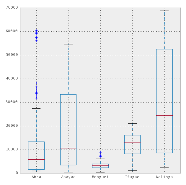
 Now plotting using pandas module can beautify the above plot into the theme of the popular R plotting package, the ggplot. To use the ggplot theme just add one more line to the above code,
And you'll have the following,
 Even neater than the default matplotlib.pyplot theme. But in this post, I would like to introduce the seaborn module which is a statistical data visualization library. So that, we have the following
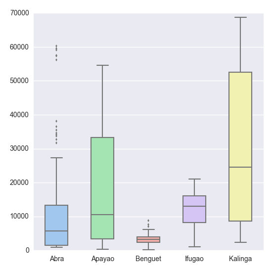 Sexy boxplot, scroll down for more.
By the way, in Python indentation is important. Use indentation for scope of the function, which in R we do it with braces
Above code might be easy to read, but it's slow in replication. Below is the improvement of the above code, thanks to Python gurus, see comments on my previous post.
- Importing the data
- Importing CSV file both locally and from the web;
- Data transformation;
- Descriptive statistics of the data;
- Hypothesis testing
- One-sample t test;
- Visualization; and
- Creating custom function.
Importing the data
This is the crucial step, we need to import the data in order to proceed with the succeeding analysis. And often times data are in CSV format, if not, at least can be converted to CSV format. In Python we can do this using the following codes:To read CSV file locally, we need the
pandas module which is a python data analysis library. The read_csv function can read data both locally and from the web.Data transformation
Now that we have the data in the workspace, next is to do transformation. Statisticians and scientists often do this step to remove unnecessary data not included in the analysis. Let's view the data first:To R programmers, above is the equivalent of
print(head(df)) which prints the first six rows of the data, and print(tail(df)) -- the last six rows of the data, respectively. In Python, however, the number of rows for head of the data by default is 5 unlike in R, which is 6. So that the equivalent of the R code head(df, n = 10) in Python, is df.head(n = 10). Same goes for the tail of the data.Column and row names of the data are extracted using the
colnames and rownames functions in R, respectively. In Python, we extract it using the columns and index attributes. That is,Transposing the data is obtain using the
T method,
Other transformations such as sort can be done using
sort attribute. Now let's extract a specific column. In Python, we do it using either iloc or ix attributes, but ix is more robust and thus I prefer it. Assuming we want the head of the first column of the data, we have
By the way, the indexing in Python starts with 0 and not 1. To slice the index and first three columns of the 11th to 21st rows, run the following
Which is equivalent to
print df.ix[10:20, ['Abra', 'Apayao', 'Benguet']]To drop a column in the data, say columns 1 (Apayao) and 2 (Benguet), use the
drop attribute. That is,
axis argument above tells the function to drop with respect to columns, if axis = 0, then the function drops with respect to rows.Descriptive Statistics
Next step is to do descriptive statistics for preliminary analysis of our data using thedescribe attribute:
Hypothesis Testing
Python has a great package for statistical inference. And that's the stats library of scipy. The one sample t-test is implemented inttest_1samp function. So that, if we want to test the mean of the Abra's volume of palay production against the null hypothesis with 15000 assumed population mean of the volume of palay production, we have
The values returned are tuple of the following values:
- t : float or array
t-statistic - prob : float or array
two-tailed p-value
The first array returned is the t-statistic of the data, and the second array is the corresponding p-values.
Visualization
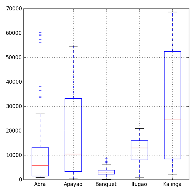
There are several module for visualization in Python, and the most popular one is the matplotlib library. To mention few, we have bokeh and seaborn modules as well to choose from. In my previous post, I've demonstrated the matplotlib package which has the following graphic for box-whisker plot,And you'll have the following,
Creating custom function
To define a custom function in Python, we use thedef function. For example, say we define a function that will
add two numbers, we do it as follows,By the way, in Python indentation is important. Use indentation for scope of the function, which in R we do it with braces
{...}. Now here's an algorithm from my previous post,
- Generate samples of size 10 from Normal distribution with $\mu$ = 3 and $\sigma^2$ = 5;
- Compute the $\bar{x}$ and $\bar{x}\mp z_{\alpha/2}\displaystyle\frac{\sigma}{\sqrt{n}}$ using the 95% confidence level;
- Repeat the process 100 times; then
- Compute the percentage of the confidence intervals containing the true mean.
Above code might be easy to read, but it's slow in replication. Below is the improvement of the above code, thanks to Python gurus, see comments on my previous post.
Comments
Post a Comment