In Statistics, we model random phenomenon and make conclusions about its population. For example, in an experiment of determining the true heights of the students in the university. Suppose we take sample from the population of the students, and consider testing the null hypothesis that the average height is 5.4 ft against an alternative hypothesis that the average height is greater than 5.4 ft. Mathematically, we can represent this as $H_0:\theta=\theta_0$ vs $H_1:\theta>\theta_0$, where $\theta$ is the true value of the parameter, and $\theta_0=5.4$ is the testing value set by the experimenter. And because we only consider subset (the sample) of the population for testing the hypotheses, then we expect for errors we commit. To understand these errors, consider if the above test results into rejecting $H_0$ given that $\theta\in\Theta_0$, where $\Theta_0$ is the parameter space of the null hypothesis, in other words we mistakenly reject $H_0$, then in this case we committed a Type I error. Another is, if the above test results into accepting $H_0$ given that $\theta\in\Theta_0^c$, where $\Theta_0^c$ is the parameter space of the alternative hypothesis, then we committed a Type II error. To summarize this consider the following table,
Let's formally define the power function, from Casella and Berger (2001), see reference 1.
Example 1. Let $X_1,\cdots, X_n\overset{r.s.}{\sim}N(\mu,\sigma^2)$ -- normal population where $\sigma^2$ is known. Consider testing $H_0:\theta\leq \theta_0$ vs $H_1:\theta> \theta_0$, obtain the likelihood ratio test (LRT) statistic and its power function.
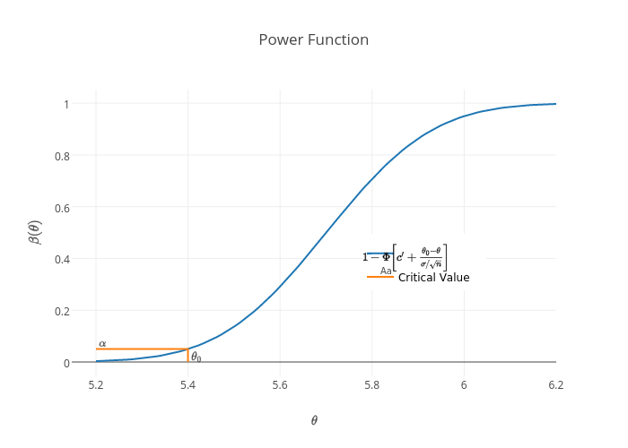
Solution: The LRT statistic is given by $$ \lambda(\mathbf{x})=\frac{\displaystyle\sup_{\theta\leq\theta_0}L(\theta|\mathbf{x})}{\displaystyle\sup_{-\infty<\theta<\infty}L(\theta|\mathbf{x})}, $$ where $$ \begin{aligned} \sup_{\theta\leq\theta_0}L(\theta|\mathbf{x})&=\sup_{\theta\leq\theta_0}\prod_{i=1}^{n}\frac{1}{\sqrt{2\pi}\sigma}\exp\left[-\frac{(x_i-\theta)^2}{2\sigma^2}\right]\\ &=\sup_{\theta\leq\theta_0}\frac{1}{(2\pi\sigma^2)^{1/n}}\exp\left[-\displaystyle\sum_{i=1}^{n}\frac{(x_i-\theta)^2}{2\sigma^2}\right]\\ &=\frac{1}{(2\pi\sigma^2)^{1/n}}\exp\left[-\displaystyle\sum_{i=1}^{n}\frac{(x_i-\theta_0)^2}{2\sigma^2}\right]\\ &=\frac{1}{(2\pi\sigma^2)^{1/n}}\exp\left[-\displaystyle\sum_{i=1}^{n}\frac{(x_i-\bar{x}+\bar{x}-\theta_0)^2}{2\sigma^2}\right]\\ &=\frac{1}{(2\pi\sigma^2)^{1/n}}\exp\left\{-\displaystyle\sum_{i=1}^{n}\left[\frac{(x_i-\bar{x})^2+2(x_i-\bar{x})(\bar{x}-\theta_0)+(\bar{x}-\theta_0)^2}{2\sigma^2}\right]\right\}\\ &=\frac{1}{(2\pi\sigma^2)^{1/n}}\exp\left[-\frac{(n-1)s^2+n(\bar{x}-\theta_0)^2}{2\sigma^2}\right], \text{since the middle term is 0.} \end{aligned} $$ And $$ \begin{aligned} \sup_{-\infty<\theta<\infty}L(\theta|\mathbf{x})&=\sup_{-\infty<\theta<\infty}\prod_{i=1}^{n}\frac{1}{\sqrt{2\pi}\sigma}\exp\left[-\frac{(x_i-\theta)^2}{2\sigma^2}\right]\\ &=\sup_{-\infty<\theta<\infty}\frac{1}{(2\pi\sigma^2)^{1/n}}\exp\left[-\displaystyle\sum_{i=1}^{n}\frac{(x_i-\theta)^2}{2\sigma^2}\right]\\ &=\frac{1}{(2\pi\sigma^2)^{1/n}}\exp\left[-\displaystyle\sum_{i=1}^{n}\frac{(x_i-\bar{x})^2}{2\sigma^2}\right],\quad\text{since }\bar{x}\text{ is the MLE of }\theta.\\ &=\frac{1}{(2\pi\sigma^2)^{1/n}}\exp\left[-\frac{n-1}{n-1}\displaystyle\sum_{i=1}^{n}\frac{(x_i-\bar{x})^2}{2\sigma^2}\right]\\ &=\frac{1}{(2\pi\sigma^2)^{1/n}}\exp\left[-\frac{(n-1)s^2}{2\sigma^2}\right],\\ \end{aligned} $$ so that $$ \begin{aligned} \lambda(\mathbf{x})&=\frac{\frac{1}{(2\pi\sigma^2)^{1/n}}\exp\left[-\frac{(n-1)s^2+n(\bar{x}-\theta_0)^2}{2\sigma^2}\right]}{\frac{1}{(2\pi\sigma^2)^{1/n}}\exp\left[-\frac{(n-1)s^2}{2\sigma^2}\right]}\\ &=\exp\left[-\frac{n(\bar{x}-\theta_0)^2}{2\sigma^2}\right].\\ \end{aligned} $$ And from my previous entry, $\lambda(\mathbf{x})$ is rejected if it is small, such that $\lambda(\mathbf{x})\leq c$ for some $c\in[0,1]$. Hence, $$ \begin{aligned} \lambda(\mathbf{x})&=\exp\left[-\frac{n(\bar{x}-\theta_0)^2}{2\sigma^2}\right]< c\\&\Rightarrow-\frac{n(\bar{x}-\theta_0)^2}{2\sigma^2}<\log c\\ &\Rightarrow\frac{\bar{x}-\theta_0}{\sigma/\sqrt{n}}>\sqrt{-2\log c}. \end{aligned} $$ So that $H_0$ is rejected if $\frac{\bar{x}-\theta_0}{\sigma/\sqrt{n}}> c'$ for some $c'=\sqrt{-2\log c}\in[0,\infty)$. Now the power function of the test, is the probability of rejecting the null hypothesis given that it is true, or the probability of the Type I error given by, $$ \begin{aligned} \beta(\theta)&=\mathrm{P}\left[\frac{\bar{x}-\theta_0}{\sigma/\sqrt{n}}> c'\right]\\ &=\mathrm{P}\left[\frac{\bar{x}-\theta+\theta-\theta_0}{\sigma/\sqrt{n}}> c'\right]\\ &=\mathrm{P}\left[\frac{\bar{x}-\theta}{\sigma/\sqrt{n}}+\frac{\theta-\theta_0}{\sigma/\sqrt{n}}> c'\right]\\ &=\mathrm{P}\left[\frac{\bar{x}-\theta}{\sigma/\sqrt{n}}> c'-\frac{\theta-\theta_0}{\sigma/\sqrt{n}}\right]\\ &=1-\mathrm{P}\left[\frac{\bar{x}-\theta}{\sigma/\sqrt{n}}\leq c'+\frac{\theta_0-\theta}{\sigma/\sqrt{n}}\right]\\ &=1-\Phi\left[c'+\frac{\theta_0-\theta}{\sigma/\sqrt{n}}\right]. \end{aligned} $$ To illustrate this, consider $\theta_0=5.4,\sigma = 1,n=30$ and $c'=1.645$. Then the plot of the power function as a function of $\theta$ is,
 Since $\beta$ is an increasing function with unit range, then
$$
\alpha = \sup_{\theta\leq\theta_0}\beta(\theta)=\beta(\theta_0)=1-\Phi(c').
$$
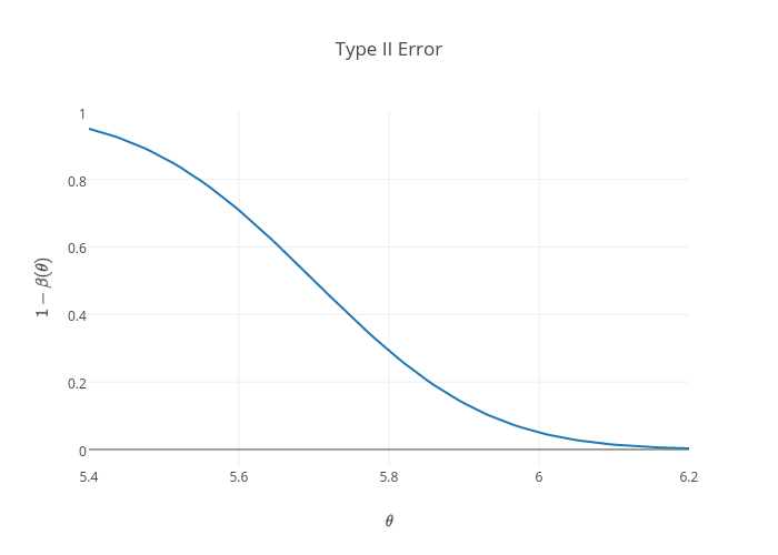
So that using values we set for the above graph, $\alpha=0.049985\approx 0.05$, $\alpha$ here is called the size of the test since it is the supremum of the power function over $\theta\leq\theta_0$, see reference 1 for level of the test. Now let's investigate the power function above, the probability of committing Type I error, $\beta(\theta), \forall \theta\leq \theta_0$, is acceptably small. However, the probability of committing Type II error, $1-\beta(\theta), \forall \theta > \theta_0$, is too high as we can see in the following plot,
Since $\beta$ is an increasing function with unit range, then
$$
\alpha = \sup_{\theta\leq\theta_0}\beta(\theta)=\beta(\theta_0)=1-\Phi(c').
$$
So that using values we set for the above graph, $\alpha=0.049985\approx 0.05$, $\alpha$ here is called the size of the test since it is the supremum of the power function over $\theta\leq\theta_0$, see reference 1 for level of the test. Now let's investigate the power function above, the probability of committing Type I error, $\beta(\theta), \forall \theta\leq \theta_0$, is acceptably small. However, the probability of committing Type II error, $1-\beta(\theta), \forall \theta > \theta_0$, is too high as we can see in the following plot,
 Therefore, it's better to investigate the error structure when considering the power of the test. From Casella and Berger (2001), the ideal power function is 0 $\forall\theta\in\Theta_0$ and 1 $\forall\theta\in\Theta_0^c$. Except in trivial situations, this ideal cannot be attained. Qualitatively, a good test has power function near 1 for most $\theta\in\Theta_0^c$ and $\theta\in\Theta_0$. Implying, one that has steeper power curve.
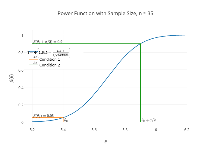
Now an interesting fact about power function is that it depends on the sample size $n$. Suppose in our experiment above we want the Type I error to be 0.05 and the Type II error to be 0.1 if $\theta\geq \theta_0+\sigma/2$. Since the power function is increasing, then we have $$ \beta(\theta_0)=0.05\Rightarrow c'=1.645\quad\text{and}\quad 1 - \beta(\theta_0+\sigma/2)=0.1\Rightarrow\beta(\theta_0+\sigma/2)=0.9. $$ Where $$ \begin{aligned} \beta(\theta_0+\sigma/2)&=1-\Phi\left[c' +\frac{\theta_0-\sigma/2-\theta_0}{\sigma/\sqrt{n}}\right]\\ &=1-\Phi\left[c' - \frac{\sqrt{n}}{2}\right]\\ 0.9&=1-\Phi\left[1.645 - \frac{\sqrt{n}}{2}\right]\\ 0.1&=\Phi\left[1.645 - \frac{\sqrt{n}}{2}\right].\\ \end{aligned} $$ Hence, $n$ is chosen such that it solves the above equation. That is, $$ \begin{aligned} 1.645 - \frac{\sqrt{n}}{2}&=-1.28155,\quad\text{since }\Phi(-1.28155)=0.1\\ \frac{3.29 - \sqrt{n}}{2}&=-1.28155\\ 3.29 - \sqrt{n}&=-2.5631\\ n&=(3.29+2.5631)^2=34.25878,\;\text{take }n=35. \end{aligned} $$ For purpose of illustration, we'll consider the non-rounded value of $n$. Below is the plot of this,
 And for different values of $n$, consider the following power functions
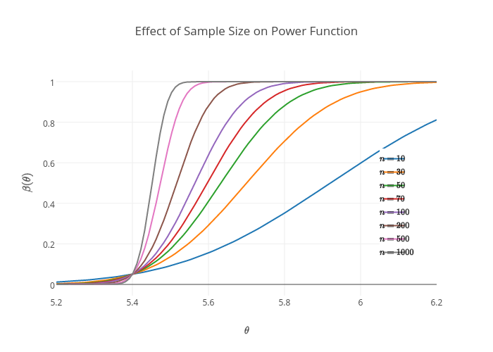 From the above plot, the larger the sample size, $n$, the steeper the curve implying a better error structure. To see this, try hovering over the lines in the plot, and you'll witness a fast departure for values of large $n$ on the unit range, this characteristics contribute to the sensitivity of the test.
| Truth | Decision | ||
|---|---|---|---|
Table 1: Two Types of Errors in Hypothesis Testing.
| |||
| Accept $H_0$ | Reject $H_0$ | ||
| $H_0$ | Correct Decision | Type I Error | |
| $H_1$ | Type II Error | Correct Decision | |
Let's formally define the power function, from Casella and Berger (2001), see reference 1.
Definition 1. The power function of a hypothesis test with rejection region $R$ is the function of $\theta$ defined by $\beta(\theta)=\mathrm{P}_{\theta}(\mathbf{X}\in R)$.To relate the definition to the above problem, if $R$ is the rejection region of $H_0$. Then we make mistake if the sample observed, $\mathbf{x}$, $\mathbf{x}\in R$ given that $\theta\in\Theta_0$. That is, $\beta(\theta)=\mathrm{P}_{\theta}(\mathbf{X}\in R)$ is the probability of Type I error. Let's consider an example, one that is popularly used in testing the sample mean. The example below is the combined problem of Example 8.3.3 and Exercise 8.37 (a) of reference 1.
Example 1. Let $X_1,\cdots, X_n\overset{r.s.}{\sim}N(\mu,\sigma^2)$ -- normal population where $\sigma^2$ is known. Consider testing $H_0:\theta\leq \theta_0$ vs $H_1:\theta> \theta_0$, obtain the likelihood ratio test (LRT) statistic and its power function.
Solution: The LRT statistic is given by $$ \lambda(\mathbf{x})=\frac{\displaystyle\sup_{\theta\leq\theta_0}L(\theta|\mathbf{x})}{\displaystyle\sup_{-\infty<\theta<\infty}L(\theta|\mathbf{x})}, $$ where $$ \begin{aligned} \sup_{\theta\leq\theta_0}L(\theta|\mathbf{x})&=\sup_{\theta\leq\theta_0}\prod_{i=1}^{n}\frac{1}{\sqrt{2\pi}\sigma}\exp\left[-\frac{(x_i-\theta)^2}{2\sigma^2}\right]\\ &=\sup_{\theta\leq\theta_0}\frac{1}{(2\pi\sigma^2)^{1/n}}\exp\left[-\displaystyle\sum_{i=1}^{n}\frac{(x_i-\theta)^2}{2\sigma^2}\right]\\ &=\frac{1}{(2\pi\sigma^2)^{1/n}}\exp\left[-\displaystyle\sum_{i=1}^{n}\frac{(x_i-\theta_0)^2}{2\sigma^2}\right]\\ &=\frac{1}{(2\pi\sigma^2)^{1/n}}\exp\left[-\displaystyle\sum_{i=1}^{n}\frac{(x_i-\bar{x}+\bar{x}-\theta_0)^2}{2\sigma^2}\right]\\ &=\frac{1}{(2\pi\sigma^2)^{1/n}}\exp\left\{-\displaystyle\sum_{i=1}^{n}\left[\frac{(x_i-\bar{x})^2+2(x_i-\bar{x})(\bar{x}-\theta_0)+(\bar{x}-\theta_0)^2}{2\sigma^2}\right]\right\}\\ &=\frac{1}{(2\pi\sigma^2)^{1/n}}\exp\left[-\frac{(n-1)s^2+n(\bar{x}-\theta_0)^2}{2\sigma^2}\right], \text{since the middle term is 0.} \end{aligned} $$ And $$ \begin{aligned} \sup_{-\infty<\theta<\infty}L(\theta|\mathbf{x})&=\sup_{-\infty<\theta<\infty}\prod_{i=1}^{n}\frac{1}{\sqrt{2\pi}\sigma}\exp\left[-\frac{(x_i-\theta)^2}{2\sigma^2}\right]\\ &=\sup_{-\infty<\theta<\infty}\frac{1}{(2\pi\sigma^2)^{1/n}}\exp\left[-\displaystyle\sum_{i=1}^{n}\frac{(x_i-\theta)^2}{2\sigma^2}\right]\\ &=\frac{1}{(2\pi\sigma^2)^{1/n}}\exp\left[-\displaystyle\sum_{i=1}^{n}\frac{(x_i-\bar{x})^2}{2\sigma^2}\right],\quad\text{since }\bar{x}\text{ is the MLE of }\theta.\\ &=\frac{1}{(2\pi\sigma^2)^{1/n}}\exp\left[-\frac{n-1}{n-1}\displaystyle\sum_{i=1}^{n}\frac{(x_i-\bar{x})^2}{2\sigma^2}\right]\\ &=\frac{1}{(2\pi\sigma^2)^{1/n}}\exp\left[-\frac{(n-1)s^2}{2\sigma^2}\right],\\ \end{aligned} $$ so that $$ \begin{aligned} \lambda(\mathbf{x})&=\frac{\frac{1}{(2\pi\sigma^2)^{1/n}}\exp\left[-\frac{(n-1)s^2+n(\bar{x}-\theta_0)^2}{2\sigma^2}\right]}{\frac{1}{(2\pi\sigma^2)^{1/n}}\exp\left[-\frac{(n-1)s^2}{2\sigma^2}\right]}\\ &=\exp\left[-\frac{n(\bar{x}-\theta_0)^2}{2\sigma^2}\right].\\ \end{aligned} $$ And from my previous entry, $\lambda(\mathbf{x})$ is rejected if it is small, such that $\lambda(\mathbf{x})\leq c$ for some $c\in[0,1]$. Hence, $$ \begin{aligned} \lambda(\mathbf{x})&=\exp\left[-\frac{n(\bar{x}-\theta_0)^2}{2\sigma^2}\right]< c\\&\Rightarrow-\frac{n(\bar{x}-\theta_0)^2}{2\sigma^2}<\log c\\ &\Rightarrow\frac{\bar{x}-\theta_0}{\sigma/\sqrt{n}}>\sqrt{-2\log c}. \end{aligned} $$ So that $H_0$ is rejected if $\frac{\bar{x}-\theta_0}{\sigma/\sqrt{n}}> c'$ for some $c'=\sqrt{-2\log c}\in[0,\infty)$. Now the power function of the test, is the probability of rejecting the null hypothesis given that it is true, or the probability of the Type I error given by, $$ \begin{aligned} \beta(\theta)&=\mathrm{P}\left[\frac{\bar{x}-\theta_0}{\sigma/\sqrt{n}}> c'\right]\\ &=\mathrm{P}\left[\frac{\bar{x}-\theta+\theta-\theta_0}{\sigma/\sqrt{n}}> c'\right]\\ &=\mathrm{P}\left[\frac{\bar{x}-\theta}{\sigma/\sqrt{n}}+\frac{\theta-\theta_0}{\sigma/\sqrt{n}}> c'\right]\\ &=\mathrm{P}\left[\frac{\bar{x}-\theta}{\sigma/\sqrt{n}}> c'-\frac{\theta-\theta_0}{\sigma/\sqrt{n}}\right]\\ &=1-\mathrm{P}\left[\frac{\bar{x}-\theta}{\sigma/\sqrt{n}}\leq c'+\frac{\theta_0-\theta}{\sigma/\sqrt{n}}\right]\\ &=1-\Phi\left[c'+\frac{\theta_0-\theta}{\sigma/\sqrt{n}}\right]. \end{aligned} $$ To illustrate this, consider $\theta_0=5.4,\sigma = 1,n=30$ and $c'=1.645$. Then the plot of the power function as a function of $\theta$ is,
Now an interesting fact about power function is that it depends on the sample size $n$. Suppose in our experiment above we want the Type I error to be 0.05 and the Type II error to be 0.1 if $\theta\geq \theta_0+\sigma/2$. Since the power function is increasing, then we have $$ \beta(\theta_0)=0.05\Rightarrow c'=1.645\quad\text{and}\quad 1 - \beta(\theta_0+\sigma/2)=0.1\Rightarrow\beta(\theta_0+\sigma/2)=0.9. $$ Where $$ \begin{aligned} \beta(\theta_0+\sigma/2)&=1-\Phi\left[c' +\frac{\theta_0-\sigma/2-\theta_0}{\sigma/\sqrt{n}}\right]\\ &=1-\Phi\left[c' - \frac{\sqrt{n}}{2}\right]\\ 0.9&=1-\Phi\left[1.645 - \frac{\sqrt{n}}{2}\right]\\ 0.1&=\Phi\left[1.645 - \frac{\sqrt{n}}{2}\right].\\ \end{aligned} $$ Hence, $n$ is chosen such that it solves the above equation. That is, $$ \begin{aligned} 1.645 - \frac{\sqrt{n}}{2}&=-1.28155,\quad\text{since }\Phi(-1.28155)=0.1\\ \frac{3.29 - \sqrt{n}}{2}&=-1.28155\\ 3.29 - \sqrt{n}&=-2.5631\\ n&=(3.29+2.5631)^2=34.25878,\;\text{take }n=35. \end{aligned} $$ For purpose of illustration, we'll consider the non-rounded value of $n$. Below is the plot of this,
Comments
Post a Comment